IESO IO File Structure

Introduction

This article documents the input-output (IO) file structure used by the Integrated Energy Systems Optimiser (IESO), a linear optimiser-based energy system modelling environment designed to support initial investigations such as options evaluation and trend analysis.

IESO’s modelling approach is described in this article. Installation and run instructions can be found in the setup guide.

IESO is called with one or two arguments: (1) a JSON file (referred to as input.json) that describes the dataset, and (2) an optional carbon constraint. The output is a file named input.ieso.json. It mirrors input.json and adds the optimisation results in place.

High-level overview

An IESO dataset defines primary demands (electricity and X commodities: heat, hydrogen, water) and the supply and flexibility options that meet them. The JSON below shows the top-level structure.

The five top-level objects are: demand (electricity and X), p2x (Power-to-X processes), generator (power generators), flex (flexibility means), and solver (linear solver summary).

The philosophy of IESO is to first define the demand and its hourly profile, and then describe how this demand is met:

• Electricity demand – whether primary (final consumption) or secondary (for battery charging or the operation of PtX processes) – is always met by the mix of available generators.
• Demand for commodity X (heat, hydrogen, water) is met by PtX processes, which consume electricity and, where relevant, heat from cogeneration plants.

Demand objects

Demand objects represent the final consumption of electricity and other commodities (heat, hydrogen, water). Each demand entry follows a consistent structure.

Demand for electricity

Demand for other commodities (heat, hydrogen, water)

General attributes

• iden – identifier (electricity, heat, hydrogen, or water)
• total – annual demand (MWh, kg, or m³ depending on commodity)
• profile – optional CSV with 8760 hourly values. May be provided as (1) a CSV file path, (2) an array of 8760 values, or (3) empty for a flat profile.
• supply_sources – PtX processes supplying the X commodity (a list of iden of PtX processes is expected here)
• var_cost_ns – penalty for unmet demand ($/MWh, $/kg, $/m³)
• l_ns – lower and upper bounds on annual unmet demand

Outputs

• output_ns – hourly unmet demand
• shadow_prices["demand_match"] – hourly shadow prices ($/unit). It corresponds to the dual variable of the demand-balance constraint. This value is defined for both electricity and commodities X (heat, hydrogen, water).
• shadow_prices["carbon_cap"] – carbon constraint shadow price ($/unit). It measures the implicit cost of relaxing the system-wide carbon emission limit by one unit. This price applies only to electricity – not to commodities X.
• shadow_prices["reliability_cap"] – reliability constraint shadow price ($/unit). It measures the marginal system cost of relaxing the reliability requirement by one unit of served electricity. This variable also applies only to electricity – not to commodities X.
• kpis["cost"] – average cost per unit of delivered output ($/unit). It is derived from the total expenditure incurred to meet the demand for electricity and commodities X, allocated to each demand category in proportion to its equivalent electricity consumption.
• kpis["emis"] – average emissions per unit of delivered output (kg CO₂eq/unit). It follows the same allocation principle as cost, i.e., emissions are distributed on the basis of electricity use.
• kpis["reli"] – reliability factor (%). It quantifies the proportion of total demand that is effectively served, providing a direct measure of system adequacy and security of supply.

Power-to-X (PtX) processes   |   Modelling approach →

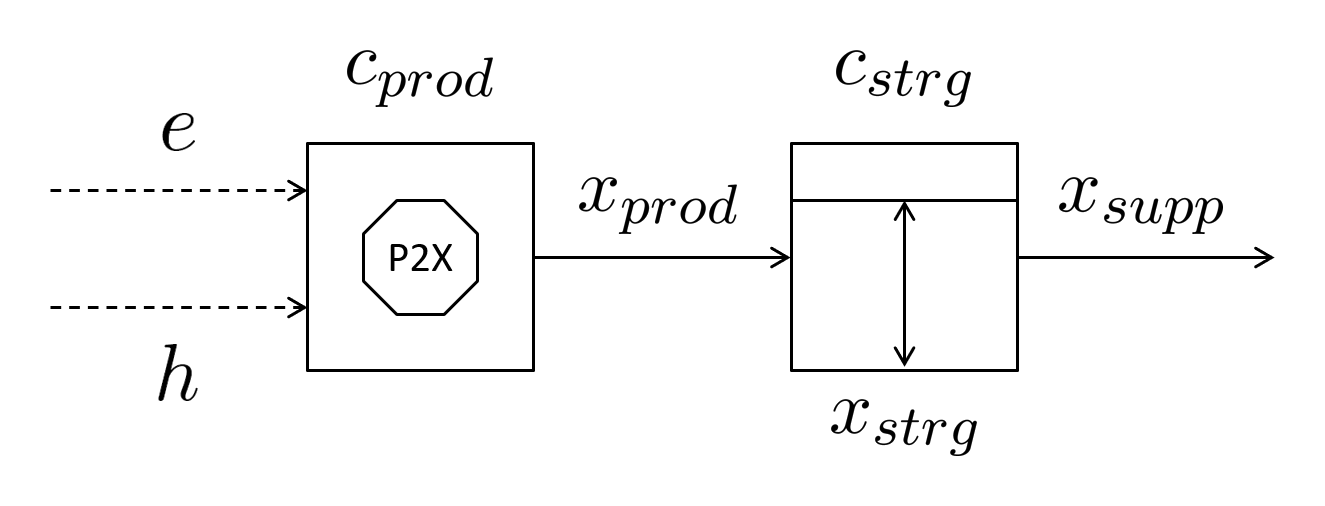
PtX processes convert electricity, and sometimes heat, into products such as hydrogen, water, or heat. Each process combines general attributes, a production unit, and a storage unit.

PtX processes are described by a consistent JSON structure.

Electricity-consuming process (e.g., RO – Reverse Osmosis)

Electricity- and heat-consuming process (e.g., MED – Multi-Effect Distillation)

General attributes

• type – elec (electric only) or elec + ther (electricity plus heat)
• temperature – required steam extraction temperature (°C, thermal processes only)
• capacity_factor – capacity factor of the plant (fraction)
• profile – optional CSV with 8760 hourly values. May be provided as (1) a CSV file path, (2) an array of 8760 values, or (3) empty for a flat profile.
• supply_sources – thermal generators eligible to supply heat in cogeneration mode (a list of iden of thermal generators is expected here)

Production unit

• c_prod – production capacity (Q/hour). Will be optimised by the solver if set to -1
• l_prod – lower and upper bounds (Q/hour)
• fix_cost_prod – fixed production costs ($ per (Q/hour) per year)
• var_cost_prod – variable costs excluding energy ($/Q)
• pow_use_elec_prod – electricity use (MWh/Q)
• pow_use_ther_prod – heat use (MWh/Q)

Storage unit

• c_strg – storage capacity (Q). Will be optimised by the solver if set to -1
• l_strg – lower and upper bounds (Q)
• fix_cost_strg – fixed storage costs ($ per Q per year)
• soc_ini – initial state of charge (fraction of c_strg)

Outputs

• x_prod – hourly production (Q/hour)
• x_strg – storage level (Q)
• x_supp – hourly supply (Q/hour)
• shadow_prices["demand_match"] – hourly shadow heat supply prices ($/MWh). Applies to thermal processes only, i.e., Power-to-X units thermally coupled to cogeneration units.

Generators   |   Modelling approach →

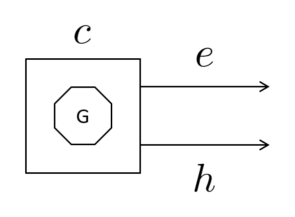
Generators represent technologies that produce electricity, heat, or both.

Generators are described by a consistent JSON structure. Dispatchable units (nuclear, coal, CCGT) may use only a capacity factor, while variable renewables (solar, wind) require hourly profiles.

Electricity-generating plant – variable (e.g., wind)

Electricity-generating plant – fully dispatchable (e.g., OCGT – Open Cycle Gas Turbine)

Cogeneration plant (e.g., CCGT – Combined Cycle Gas Turbine)

General attributes

• type – elec or elec + ther (thermal generators eligible to supply heat in cogeneration mode)
• profile – empty for dispatchable units, required for renewables (CSV, 8760 values). May be provided as (1) a CSV file path, (2) an array of 8760 values, or (3) empty for a flat profile.
• capacity_factor – capacity factor of the plant (fraction)
• l_prod – lower and upper bounds (MW)
• c_prod – installed capacity (MW). Will be optimised by the solver if set to -1

Costs and emissions

• fix_cost_prod – fixed costs ($/MW/year)
• var_cost_prod – variable costs ($/MWh)
• var_emis_prod – emissions (kg CO₂eq/MWh)

Cogeneration parameters

• turbine_t_p – turbine inlet temperature (°C) and pressure (bar)
• condenser_p – condenser pressure (bar)

Outputs

• a, b – coefficients describing electricity-heat trade-off (calculated by IESO)
• e_prod – hourly electricity production (MWh)
• h_prod – hourly heat production (MWh)

Flexibility means   |   Modelling approach →

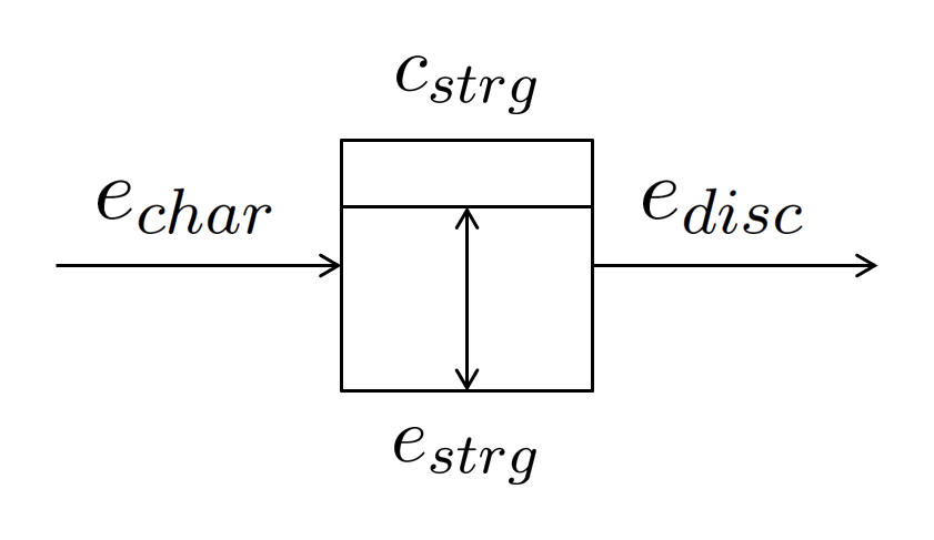
Flexibility means represent energy storage systems such as batteries or pumped hydro. They allow electricity to be shifted in time with round-trip efficiency losses.

Flexibility means are described by a consistent JSON structure.

General attributes

• fix_cost_strg – annual fixed costs ($/MWh/year)
• hours_of_storage – storage duration at maximum discharge
• round_trip_efficiency – round-trip efficiency (in [0, 1])
• soc_ini – initial state of charge (fraction of c_strg)
• l_strg – lower and upper bounds (MWh)
• c_strg – storage capacity. Will be optimised by the solver if set to -1

Outputs

• e_strg – energy stored (MWh)
• e_char – charging power (MW)
• e_disc – discharging power (MW)

Solver object   |   More about the optimisation process →

The solver object provides diagnostics for each optimisation run: status, run time, and problem size.

Outputs

• stat_succ – solver status (-1 initial, 0 failed, 1 success)
• stat_time – elapsed time (seconds)
• stat_capa – number of capacity variables
• stat_outp – number of output variables
• stat_cons – total number of constraints